
Learning how to use pivot tables in Microsoft Excel is one of the most powerful and useful features of Excel. With very little effort, you can use a pivot table to build beautiful reports for large data sets.
A pivot table is a summary of a large data set that typically includes the total figures, average, minimum, maximum, etc.
Let’s say you have sales data for different regions, with a pivot table, you can summarize the data by region and find the average, etc.
Pivot tables allow us to analyze, summarize, and display only relevant data in our reports.
Use a pivot table in Excel
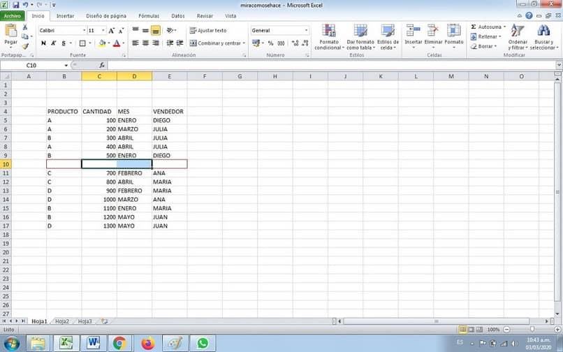
Before you start using PivotTables in Microsoft Excel, you need to make sure that your source data doesn’t have any blank rows.
This is not to say that you can’t have some blank cells, but an entire blank row will cause problems. In the spreadsheet that you can see below, there is a blank row, this would be a problem.
You must prepare the spreadsheet to ensure that it consists of immediate data that you will use.
To quickly remove them:
- Go to Home > Find > Go To Special > Blanks > Delete Rows.
- Now simply click on one of the cells in the source data and click the “Insert” tab.
- Once there, find the “Tables” group and click on “Pivot Table”. The wizard to create a pivot table should appear.
Remember that when you preselect the data, the range is shown in the upper section of the wizard. If you want you can modify it, but as long as the base data has an adjacent range, it should be correct.
That is why you must make sure that there are no blank rows before starting the process.
- Next, leave the PivotTable placement option on the default “New Worksheet” and click OK.
- Excel will open a new worksheet and place the PivotTable there. It may not seem like a big deal. but you have created your own pivot table.
Right now the blackboard is blank. You should also see something new on the right edge of this worksheet. That’s where you’ll find the available PivotTable fields and the four areas where you can place them.
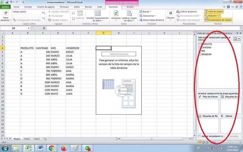
In case you don’t see
Click inside the pivot table on the left side of this worksheet. If you still don’t see the PivotTable fields, you should check the “Display” group on the “Analyze” tab to make sure “Field List” is selected.
Make sure the background is dark gray by clicking on “Field List”. This way you can use pivot tables in Microsoft Excel.
The most common problems when using pivot tables in Excel
The errors that we can find when using pivot tables in Excel can be various and for different problems. Here we will mention a couple of the most common problems:
Use numbers as text
Sometimes it happens that when the data is exported externally, the numbers that come in the file have the text format.
Regardless of whether they are seen as numbers, the Excel program interprets them as if they were text and for this reason it does not perform the addition task. It should be noted that if you wish you can give your spreadsheet a name so that you can identify it respectively.
Use past versions of Excel
It is recommended to use the most current versions of Excel, either to make pivot tables or to do any other type of work.
Older versions, such as 2003, have a different format, so you may get an error when trying to use a file created in newer versions of Excel.