
The Excel tool allows us to process different types of data; Sometimes we will need to hide the information in a cell, because of its content or to hide a formula in an Excel sheet. So today we will teach you how to hide data in Excel using conditional formatting.
How to hide data in Excel and what is its use?
We can hide rows or columns, even a specific cell or hide an Excel sheet with a macro. There are 2 ways to prevent content from being visible, altering the size of the cells or camouflaging the text with the same background color.
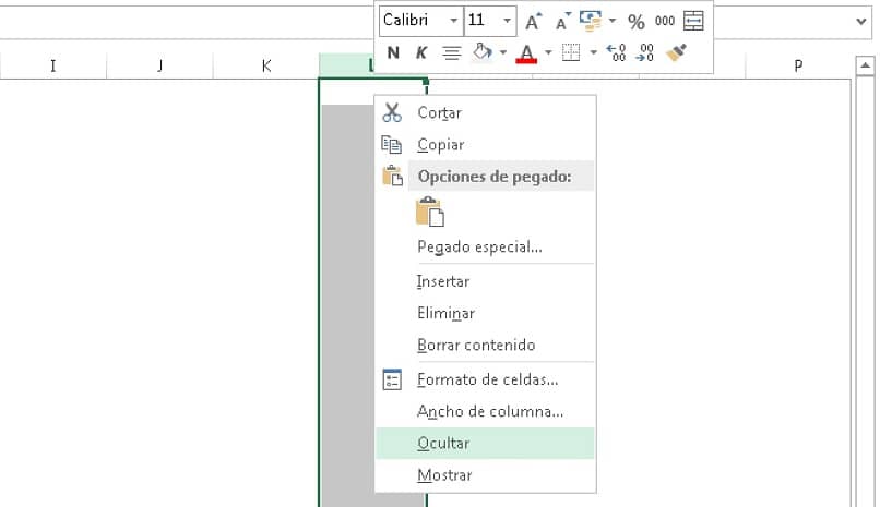
For that you just have to make the selection, and go to “Home > Cells > Format > Visibility > Hide and show”; In this option we can choose between hiding and displaying the marked row or column. You can also display the context menu on the column or row and choose the Hide option.
We can camouflage the cells by selecting the “Home > Font > Font Color” option, where we can change the text color to white. If you prefer to change the cell background, you should go to “Home > Cells > Format > Protection > Format cells > Fill”.
These methods will leave the data hidden indefinitely. But conditional formats are the best option, to show them when a condition that you have defined yourself is met; its implementation in very easy.
What is conditional formatting?
It is a tool located in “Home > Styles > Conditional formatting”, which will change the appearance or style of one or several cells, as long as a criterion defined by a rule is met.
There are 6 types of rules to apply a format to cells, depending on the value or formula they contain; in turn, each rule allows you to apply styles to a table or cell in Excel (font type and size, borders, background colors, 2 or 3 color scale, data bars and even icons).
It is possible to change the color of a cell with conditional formatting. For example, a cell can be marked red when the value of a grade based on 10 is less than 5 (indicating that a student has failed). The variety of styles and criteria that we can define are almost infinite.
How to hide data in Excel using conditional formatting?
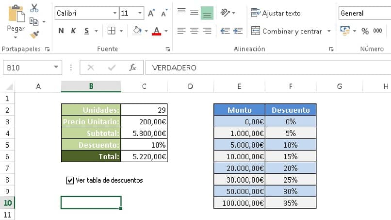
The best way to understand how this is done is through an example. First we will make a sales table, with the number of units and unit price of a product, as well as the total and subtotal of the sales made.
We will build another table with a relationship of discounts according to the number of products sold; and we want to hide or show this second table, using a conditional format that will be activated by pressing a checkbox.
We will have to make the Developer Tab visible in “File > Excel Options > Customize Ribbon > Main Tabs > Developer”. We place the checkbox in an area close to the sales table in “Developer > Insert > Form controls > Checkbox”.
Now we link the box with a cell to save its state (if it is activated it will show TRUE and if it is deactivated its will be FALSE). For that we right click on the box and select “Control format”; A window will open where we will place the chosen cell, for example B10.
We will create a rule that takes the value of cell B10 to show or hide the discount table, depending on whether the box is checked or not. For that we select the entire range of cells of the table to hide and go to the option “Home > Styles > Conditional formatting > New rule”.
In the window that opens, we select the last option “Use a formula that determines the cells to apply formatting”, we enter the formula =$B$10=FALSE and we finish with “OK”. With this, we have defined a rule that will make the table invisible until the checkbox is checked.
Now that you know how to hide data with conditional formatting, your work in Excel will be more dynamic. If you liked this post, make your comment and share it with your contacts to continue growing as professionals.


