The well-known Microsoft Office Excel tool is essential in practically any office around the world. This peculiar tool allows a multitude of functions, which is why knowing how to make a Finder in Excel is one of those things that you should know to facilitate the use of the application.
In any case, the process that we will teach you today should not be confused with searching for words in an interval or range of cells and highlighting them in Excel, on the other hand, the one indicated is also a perfectly possible process.
As we indicated before, with Excel work functions are made easier, with this useful tool we can organize enormous amounts of information, make complicated calculations in an instant and observe the development of our work or company.
In this tutorial we will teach how to make an internal search engine that will further exploit all the exceptional functions that we have in Excel, an action that added to searching for values and finding a number in a column, can become quite useful to maintain order in your tables.
How to make a search engine in Excel
To make a search engine in Excel it is necessary to first have an organized table. These types of search engines are used precisely to search for specific data in databases of considerable extension.
To make a search engine in a table follow these steps:
There are many ways to make a browser in Excel, however, the following method is applicable to almost any type of table. Today we will focus on the most basic data tables, but it is also possible to search for data in two or more Excel sheets.
Make a Finder in Excel (First part)
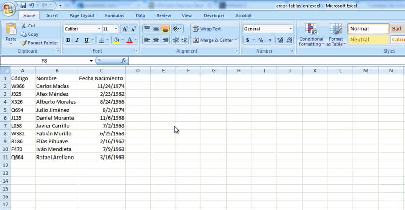
- This time we will focus on a table of basic user data. Our purpose will be to enter the user’s code (which for other purposes could well be the DNI, ID card or identification card number) so that the user’s information is shown to us, which in this case will be the Name and Date of birth .
- The first step is to create a header similar to the one that integrates the data, in our case it would be to make one that includes the columns Code, Name and Date of Birth, in another place in the table. For practical purposes we will choose from column F, but no matter the place, you can choose the one that seems best to you.
- The next step is to open the Formulas option. In this tab you will need to open Search and Reference.
Make a Finder in Excel (Second part)
- In Search and reference is the formula that we need “Search” click on it. A new tab will pop up that presents us with two options, select the searched value: Vector.
- There are three factors here that you need to define: Lookup_Value, Compare_Vector, and Result_Vector.
- Lookup value is the lookup object, in this case it is the code. Click on the blank space of Value_lookup and then on the table where you will write to search. In our case it would be just below the extra header we’ve created, specifically under the Code section.
- Comparison value, as its name indicates, is the value that will be compared with the search value. In this case we are interested in user codes. Therefore, here you must select all existing user codes. Drag from the first to the last.
- Result value is what will be displayed after entering and comparing a code. In this case we will require the name. For this, select the entire name column and click OK.
- After this, when looking for a value, in this case a user code, the name of said user will be reflected in our new header.

You can also apply the search engine to other columns
- For it to show us information from other columns, it is as simple as copying the formula and rethinking it. In this case you must copy the Name formula, which is the one we will use in the Date of Birth column.
- To this formula, which in our case should be something like “LOOKUP(F3;TABLE2 [CÓDIGO];3TABLE2[NOMBRE])” we will give you copy, then proceed to paste it in Date of Birth of the new header.
- After this, change the name to “=LOOKUP(F3,TABLE2 [CÓDIGO];TABLE2[FECHA NACIMIENTO])”.
- Doing this process, when writing the code of a user, the information of Name and Date of Birth will appear. For larger tables, the procedure is the same, you can change the formula, but always modifying the second value, that is, the result.
With the above tutorial on how to make a Finder in Excel, you will be able to easily access data from large tables. It is especially useful for databases of considerable length, such as job payrolls or student notes. Apply this useful Excel tool right now!
In turn, using the VLOOKUP or HLOOKUP function in an Excel spreadsheet is often very useful to extend its capabilities when using this popular application, seeing that it is relatively similar to the function that we discussed in the previous guide.


